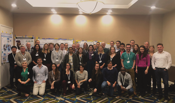
The synthesis and intercomparison of ocean carbon uptake in CMIP6 models Workshop was held December 8-9, 2018 in Washington, DC.
View or Download Workshop Report (PDF)
The objectives of this workshop were:
- Summarize high profile CMIP5 Ocean Carbon Uptake analyses and challenges, as well as the planned suite of CMIP6 experiments
- Summarize new observational constraints, including GLODAPv2, SOCAT, SOCCOM, GO-SHIP, community observational synthesis efforts such as Obs4MIPs, ocean carbon inversions, and atmospheric observations of CO2 and oxygen
- Modeling center reports on model formulation and preliminary analysis of simulated regional and global patterns in heat/carbon/tracer uptake in CMIP6 experiments
- Discuss mechanisms of heat/carbon/tracer uptake differences across models and observations towards linking physical and biogeochemical drivers and their impact
- Discuss tools and techniques that can lower barriers to analysis

Agenda and Presentation Slides
SATURDAY, DECEMBER 8
8:00 Coffee/registration
8:20 John Dunne (NOAA/GFDL) Goals, logistics and highlights of applicant responses
8:30 Matthew Long (NCAR) Introduction of community tools for model and data analysis
1) Summarize high profile CMIP5 Ocean Carbon Uptake analyses and challenges.
8:55 James Orr (IPSL) High profile summary of CMIP5/AR5 and CMIP6/ AR6
9:15 Forrest Hoffman (ORNL) Nonlinear interactions between climate and CO2 drivers of marine and terrestrial carbon cycle changes
9:40 Galen McKinley (Columbia) Forced changes and internal variability in the ocean carbon sink
10:05 Nicole Lovenduski (UC Boulder) Predicting near-term changes in ocean carbon uptake
10:30 Discussion - Make sure everybody knows the challenges and opportunities, the timeline, and can identify the resources/experts available in the room to make progress.
10:50 Coffee Break
2) Summarize new observational constraints including GLODAPv2, SOCAT, SOCCOM, GO-SHIPS, community observational synthesis efforts such as Obs4MIPs, ocean carbon inversions, and atmospheric observations of CO2 and oxygen
11:10 Nicholas Gruber (Remote - ETHZ) Observational constraints on the global ocean uptake of anthropogenic CO2
11:35 Peter Landschützer (MPI) Observation-based estimates of the regional and global ocean carbon sink
12:00 Timothy DeVries (UC Santa Barbara) Ocean Carbon Inverse Modeling
12:25 Break for lunch
1:10 Maciej Telszewski (IOCCP) Community Ocean Carbon Observational Synthesis
1:35 Abhishek Chatterjee (NASA/GSFC) Satellite based Ocean Carbon Observations
1:50 Carolina DuFour (McGill) Air-sea CO2 fluxes in the Southern Ocean: lessons learned from the comparison between CMIP5 models and SOCCOM data
2:15 Ariane Verdy (SIO) Data assimilation of carbon and other biogeochemical constraints in the Southern Ocean State Estimate
2:40 Coffee Break
3:00 Adrienne Sutton (NOAA/PMEL) Magnitude and timing of ocean carbon uptake variability constrained by seawater pCO2 time series observations
3:25 Rik Wanninkof (NOAA/AOML) How (well) do models calculate air-sea fluxes
3:50 Discussion - Inventory of what new observational and modeling analyses can be done and are planned
4:30 Lightning talks on poster presentations
5:30 Evening Poster Reception
SUNDAY, DECEMBER 9TH
8:00 Coffee/registration open
3) Modeling center reports on model formulation and preliminary analysis of the CMIP6 models in their regional and global patterns in heat/carbon/tracer uptake
8:30 John Dunne (NOAA/GFDL) GFDL’s Contributions to CMIP6
8:50 Matthew Long (NCAR) NCAR’s Contributions to CMIP6
9:10 Anastasia Romanou (NASA/GISS) GISS Contributions to CMIP6
9:30 Jim Christian (Fisheries and Oceans Canada) Recent developments in ocean biogeochemistry in the Canadian Earth System Model
9:50 James Orr (IPSL) Progress report from IPSL for CMIP6
10:10 Discussion of CMIP6 models and experiments compared to CMIP5 models and experiments and the timeline for CMIP6/AR6
10:40 Coffee Break
4) Discuss mechanisms of heat/carbon/tracer uptake differences across models and observations towards linking physical and biogeochemical drivers and their impacts
11:00 Andrea Fassbender (MBARI) Sensitivity of the ocean carbon sink to natural and anthropogenic carbon cycle interactions
11:25 Laure Resplandy (Princeton) Systematic deficiencies in ocean transport impact land and ocean carbon sinks
11:50 John Krasting (NOAA/GFDL) Resolution-dependent patterns of heat and carbon uptake in GFDL’s OMIP and OMIP-BGC simulations
12:15 Discussion and breakout group assignments
12:40 Break for Lunch
1:20 Split into three Breakout groups previously assigned with identical sets of questions for brainstorming
3:20 Coffee Break
3:40 Report back from each of the breakout groups
5:00 Conclusion/writing assignments
Key Definitions related to CMIP6 Models
(living document, click for latest updates or to comment)
OCEAN COMPONENT OF EARTH SYSTEM MODELS VS. OCEAN ONLY HINDCAST
Global coupled ocean-ice-land-atmosphere models are commonly known as “earth system models” or “climate models”. These models are typically forced only with influences external to the coupled climate system i.e. solar radiation, volcanic aerosols, and greenhouse gas concentrations. If the carbon cycle is explicitly represented, then greenhouse gas emissions would be specified and the carbon cycle will determine exchanges with the ocean and the land, and thus the model will determine the atmospheric CO2 concentration. CMIP6 models are earth system models.
In an earth system model, the state of the internal variability for the historical period is not prescribed so that it is the same as the observed. The internal variability of an earth system model is the emergent result of the coupled interactions of the system. One expects the statistics of this variability to be consistent with the historical observations, but the timing and phasing will not be. As an example, one expects the earth system model to have El Niño events occurring every 5 to 7 years, but one does not expect them to occur in 1997-98. Thus, to compare results of an earth system model to observations, one must take care that the comparisons are reasonable given the expected different states of internal variability as simulated and as observed. One rule of thumb is that averaging of 20-30 years, or 20-30 members of an ensemble of simulations is needed to get a coupled model field that can be compared to mean observations.
In order to estimate internal variability as it occurred in the historical period, the approach used is to force an ocean model with historical atmospheric reanalyses (reanalyses are atmospheric models constrained with observations so as to offer a best-estimate of the historical atmospheric state). This is an ocean-only hindcast simulation. The ocean model used may be identical to the ocean component of the earth system model, but the key difference is that the internal variability is an estimate of the actual variability. Thus, in an ocean-only hindcast simulation, one does expect El Niño to occur in 1997-98. Thus, it makes sense to make direct comparisons between observations and ocean-only hindcast simulation for the same years.
INTERNAL VARIABILITY
Ocean internal variability are deviations on all timescales from a steady repeating seasonal cycle. This is variability in circulation of all types, El Nino and other modes of climate variability, and also in ecology or biogeochemistry. In the case of an ocean-only hindcast model, the simulated internal variability is an estimate of the actual historical internal variability. Internal variability is also found in earth system models, but then its phasing is not expected to align with historical observations. Internal variability is often called “natural variability” so as to distinguish it from trends driven by external forcing.
LARGE ENSEMBLES
Large ensembles of earth system models are earth system models that are run repeatedly with small perturbations to initial conditions. These are used to estimate the full spread of potential internal variability in any represented variable and at any point in the past or future.
FORCED RESPONSE
We are interested in separating internal variability from trends due to anthropogenic forcing. A great benefit of earth system models run in large ensemble mode is that the average response of many ensembles can be taken as an estimate of this forced response, and the remaining spread across ensemble members is an estimate of the range of potential internal variability.
ESM HISTORICAL VS. HISTORICAL
In CMIP5 and CMIP6, a coupled model forced with prescribed atmospheric CO2 concentrations is an historical simulation. If the forcing is CO2 emissions and there is an active carbon cycle that then determines the atmospheric CO2 concentrations, this is called ESM historical.
PREDICTION VS. PROJECTION
Future climates are predicted on short time scales (up to 3 years) and projected on longer time scales using global coupled ocean-ice-land-atmosphere models. Short-term climate prediction works in a similar fashion to a weather forecast: Its skill depends on how well we estimate the initial state. Climate projections employ greenhouse gas emission scenarios, which are based on assumptions about future population growth and emissions per capita. Uncertainties about these projections derive firstly from the scenario uncertainty, secondly from the model uncertainty (error), and finally from internal variability, which a model never reproduces exactly. For both predictions and projections, coupled ocean-ice-land atmosphere models are required.


